broadcasting

Topics

• linear algebra
• matrices

Broadcasting is a mechanism that allows you to perform operations between arrays of different shapes. Without broadcasting, you can only do element-wise ops (add, multiply, etc.) on arrays that have exactly the same shape. In practice, you often want to add a 1D array (say, a bias vector) to every row of a 2D matrix, or add a scalar to an entire array. Broadcasting lets you do that directly. ​

Libraries like numpy, or pytorch follow specific rules to determine if shapes are compatible for broadcasting. They compare the dimensions of the two arrays starting from the rightmost, or trailing, dimension. Dimensions are compatible:

• if they are equal or
• if one of them is 1 (broadcasting virtually repeats that array along that axis to match the other’s size)

If one array has fewer dimensions, it’s conceptually padded with dimensions of size 1 on the left until the number of dimensions matches.

# broadcasting error
 
from numpy import array
A = array([
[1, 2, 3],
[1, 2, 3]])
 
b = array([1, 2])
 
# attempt broadcast: FAILS!
# A: 2x3, B: 1x2, last dims don't match
C = A + b

Note

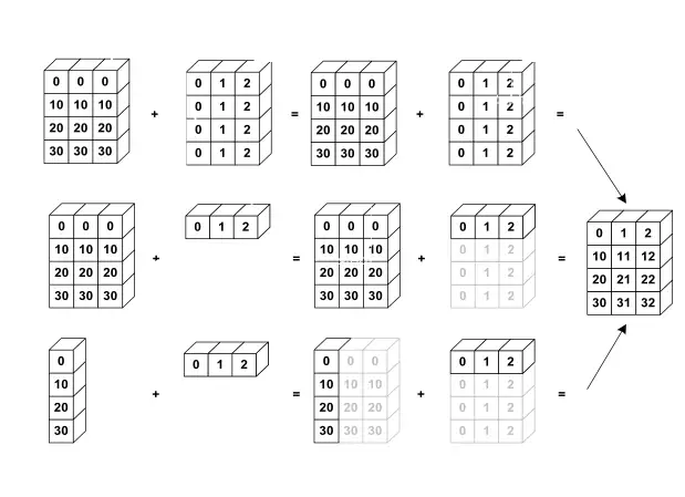
How it works (conceptually): When performing an operation between two arrays of different shapes that satisfy the broadcasting rules, the smaller array is conceptually “stretched” or “replicated” to match the shape of the larger array. This stretching happens automatically and efficiently without actually creating copies of the data in memory. The operation is then performed element-wise on the expanded shapes.

Operation	Example shapes	What happens
Scalar + array	( ) + (m, n)	Scalar treated like shape (1,1), broadcast to (m,n) → adds to every element.
1D + 2D (match columns)	(n,) + (m, n)	1D array seen as (1, n), broadcast to (m, n) → adds each row of the matrix.
2D + 2D (same shape)	(m, n) + (m, n)	Shapes match → element-wise addition/subtraction/multiplication, etc.

import numpy as np
 
A = np.array([[1,2,3],
              [4,5,6],
              [7,8,9]])    # shape (3,3)
b = np.array([10,20,30])  # shape (3,)
C = A + b  # b broadcast to (3,3)
# Result:
# [[11, 22, 33],
#  [14, 25, 36],
#  [17, 28, 39]]
 
D = A * b
# Result:
# [[ 10, 40,  90],
# [ 40, 100, 180],
# [ 70, 160, 270]]

Benefits:

• Simplifies code by removing the need to manually create larger arrays with duplicated values to match dimensions
• Improves efficiency by avoiding unnecessary memory allocation and computation compared to manual replication

Related